
Accurately identifying patients in rare disease markets is critical, both for improving patient outcomes and achieving commercial success. On the clinical side, limited disease awareness often leads to delayed diagnoses or misdiagnoses, preventing patients from receiving timely, appropriate care. Commercially, the challenge lies in pinpointing small, dispersed patient populations and the healthcare providers who treat them. Without this visibility, it can be very challenging to get important therapies to the right patients. Enhancing patient identification capabilities not only accelerates the path to diagnosis and treatment but also supports more targeted and effective engagement strategies and resource allocation.
Claims data remains a widely used source for identifying patients, particularly in rare disease markets. However, several challenges can limit its effectiveness. These include incomplete data capture, inconsistent patient stability, and the underutilization of approved ICD-10 codes. This brief case study explores how to address the latter issue by using a predictive methodology that leverages the clinical characteristics of patients already diagnosed with the appropriate ICD-10 code. This can help identify individuals who may be misdiagnosed or remain undiagnosed, ultimately expanding visibility into the true patient population.
Model Overview and Selection
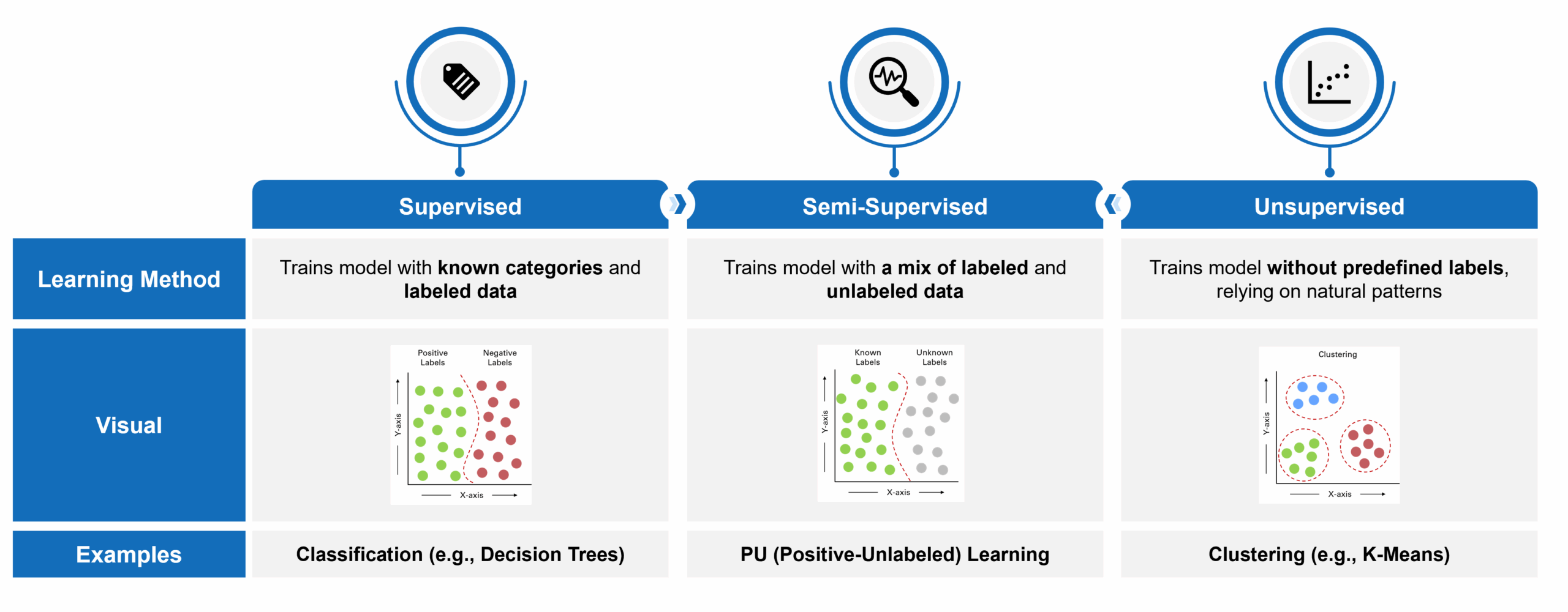
Machine learning has become one of the most powerful tools for identifying undiagnosed or misdiagnosed patients in rare diseases – areas where traditional brute force approaches often fall short. These models excel at detecting complex patterns across large volumes of data. In addition, they can process data with a high dimensionality of features (e.g., such as diagnosis and procedure codes and claims data in general, which includes a large number of discrete patient characteristics across a longitudinal medical history). However, machine learning is not a one-size-fits-all solution. The choice of model depends heavily on the type and quality of available data. Models typically fall into one of three categories:
- Supervised: Trains on fully labeled datasets with known outcomes. In this case, “labeled” means that patients can be tagged as having a certain characteristic (or not). Take lung cancer, for example, where not all patients are explicitly diagnosed in the claims data. Those with a lung cancer diagnosis code are considered “labeled” and those without are “unlabeled.”
- Semi-Supervised: Leverages a combination of labeled and unlabeled data.
- Unsupervised: Identifies natural patterns without relying on predefined labels.
In a recent project, a newly approved ICD-10 code for a rare disease enabled us to identify a subset of confirmed patients. However, due to limited physician adoption of the new code, the broader claims dataset contained a large volume of patients who were either misdiagnosed, undiagnosed, or unrelated to the disease – creating a mix of known positives and unlabeled cases. Given this data structure, a semi-supervised learning approach was most appropriate and allowed us to train a model that could extend learnings from the known cohort to identify likely undiagnosed patients across the dataset.
Common semi-supervised approaches for us to choose from included:
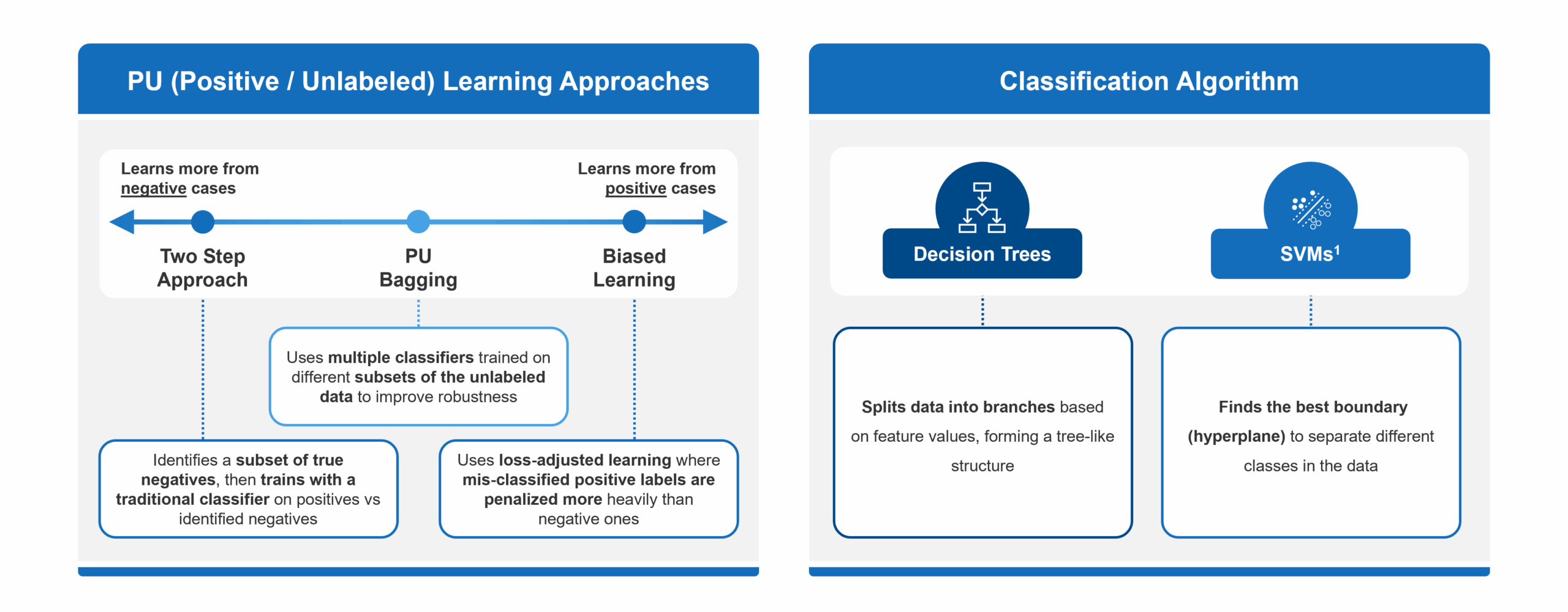
- Biased Learning: When using this approach, a model assumes that all unlabeled examples are negative. This can often lead to false negatives, which is especially problematic when many true cases remain undiagnosed.
- Two-Step Methods: These methods attempt to correct for the drawbacks of Biased Learning by identifying a subset of reliable negatives before training a model. However, they can be highly sensitive to how those negatives are selected and may still overlook hidden positives.
- PU Bagging: This technique provides a more balanced and reliable framework for identifying undiagnosed patients in rare diseases. It avoids making strong assumptions about unlabeled data and creates an ensemble of models trained on different random subsets of the unlabeled pool, minimizing the impact of mislabeling and reducing overfitting.
In essence, PU Bagging helps to average out individual model misclassifications, ensuring that predictions are not dominated by a few erroneous samples. For us, this approach increased robustness and improved recall, making it particularly effective for our rare disease situation, where identifying every potential patient can have meaningful clinical and commercial value.
However, there is another key consideration to address: the type of underlying classification algorithm to use within the selected approach. Two common algorithms include:
- Decision Trees: A flowchart-like model that splits data into branches based on feature values, leading to decisions at the “leaves.”
- Support Vector Machines (SVMs): Seeks to determine the best way to split different types of data apart, no matter how many ways you describe each item. In other words, it finds the optimal boundaries (or “hyperplanes”) that separate classes in a high-dimensional data space.
Within a PU bagging framework, decision tree classifiers are generally better suited than SVMs, particularly in our use case of working with claims data to identify undiagnosed rare disease patients. Decision trees are naturally robust to noisy data, can handle high-dimensional feature spaces like diagnosis and procedure codes, and require less preprocessing. Their interpretability also makes them more transparent and easier to validate – an important consideration in healthcare settings. In contrast, SVMs can be sensitive to mislabeled data, require careful tuning of kernels and hyperparameters, and often struggle to scale efficiently with large, sparse datasets typical of claims. Since PU bagging relies on training many models across bootstrapped samples of noisy unlabeled data, decision trees offered faster training times and better tolerance for uncertainty; thus was a more practical and effective base learner in this context.
PU Bagging Model Approach
Our PU bagging model leveraged three core components:
- Bootstrap Aggregation
- Decision Trees
- Ensemble Learning
First, bootstrap aggregation (or bagging) involved repeatedly sampling subsets of the data, combining known positive patients with randomly selected unlabeled patients, to introduce variability and reduce overfitting. Next, decision trees were used as the base classifiers within each sample. Since different trees made different assumptions about the negatives, they learn slightly different patterns. Finally, the model applied ensemble learning by aggregating predictions across all decision trees, which produced a more stable and accurate outcome than any individual model. Together, these components allowed the PU bagging approach to effectively surface likely mis- or undiagnosed patients, even in our data environment that was marked by uncertainty and limited labeled examples.
To break out these components in further detail, bootstrap aggregation, or bagging, is a foundational technique in PU bagging that enhanced our model’s robustness. It did so by generating multiple training datasets by randomly sampling the unknown patients from the larger unlabeled population. Each resampled dataset contained all available positives (i.e., the known patients stayed consistent from model to model) and a different subset of unlabeled patients, treating the latter as temporary negatives. By training unique decision trees on each of these bootstrap samples, the model learned different perspectives on the underlying data distribution. This process injects diversity into the model training phase, helping to smooth out noise introduced by mislabeled or ambiguous data points.
A critical question in our PU bagging framework was selecting the optimal decision tree hyperparameters and determining how many trees to include in the ensemble. We began by tuning key parameters – such as how many decisions the tree was making – to strike a balance between training and testing accuracy, thereby avoiding overfitting (which can occur when an algorithm fits so closely to its training data that a model is significantly hampered in making good conclusions from anything other than the training data itself) or underfitting (which describes a data model that can’t properly discern the relationship between input variables and output variables, which drives up error rates on both training data and new, unseen data). Each resulting decision tree was then combined into one overarching ensemble model, capable of generalizing unseen data.
Because several decision trees exhibited similar training and testing metrics, we adopted an iterative approach to identify the ideal ensemble size of underlying decision trees. By incrementally adding trees and evaluating ensemble performance, we were able to determine the right mix of trees that offered the optimal trade-off between accuracy and computational cost. If this was not completed, the addition of more trees would introduce unnecessary complexity and processing overhead without meaningful gains in predictive power.
After selecting optimal ensemble decision trees, our model gave us the flexibility of selecting an appropriate probability threshold (e.g., the percent confidence that the patient was tagged appropriately), which is essential for translating raw prediction scores into meaningful patient classifications. By fine-tuning the threshold to allow for greater control of the sensitivity of predicted patients, we had the ability to further validate the model through both similarity to known patients and available epidemiological (EPI) data, which we will cover in the next section.
Model Validation
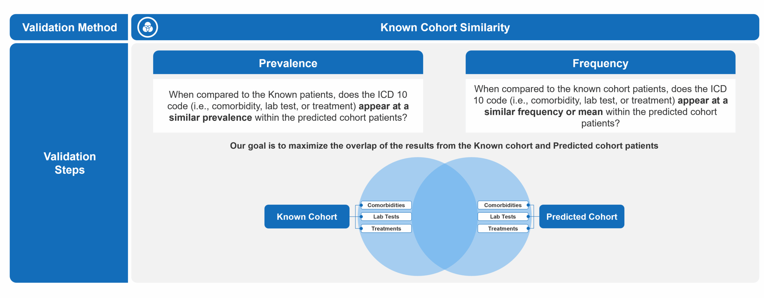
To determine the ideal probability threshold for patient prediction, we employed two complementary validation techniques. The first involved comparing incremental predicted patients to the known diagnosed cohort to identify a threshold at which meaningful differences began to emerge. The second leveraged external EPI research to estimate the expected total patient population. By combining known and predicted patients into a single cohort and applying projection factors based on claims data capture rates, we were able to assess alignment with the estimated disease prevalence and further refine the optimal threshold.
In the first approach, we analyzed the prevalence and frequency of key clinical markers, lab tests, and treatments – across both the known and predicted patient cohorts. Our goal was to maximize similarity between the two groups, under the assumption that a well-performing model would surface patients with clinical characteristics similar to those already diagnosed. We completed this by defining what constituted signification deviation from the predicted cohort to the known. Ultimately, we were able to pinpoint at what probability threshold the divergence from the known cohort became increasingly pronounced to establish a reasonable lower bound for inclusion.
To validate this further, we incorporated EPI-based prevalence estimates. By aggregating known and predicted patients at different thresholds and applying conservative, base, and optimistic projection factors – accounting for known limitations in claims capture – we triangulated the appropriate probability threshold that offered the most reliable and balanced result. This cutoff aligned with expected prevalence estimates while preserving strong clinical consistency with the known population.
Selecting the appropriate threshold also allowed us to align the model output with broader strategic objectives. In this case, the client prioritized higher recall to maximize the identification of potential patients – even at the expense of some false positives – making a slightly lower threshold more desirable. The probability threshold thus became a critical tuning lever: not only optimizing the model’s predictive reliability but also enabling downstream efforts, such as field team targeting or educational outreach, to focus on the most clinically relevant and commercially meaningful patients.